Black Box Variational Inference for Logistic Regression
Published:
A couple of weeks ago, I wrote about variational inference for probit regression, which involved some pretty ugly algebra. Although variational inference is a powerful method for approximate Bayesian inference, it can be tedious to come up with the variational updates for every model (which aren’t always available in closed-form), and these updates are model-specific.
Black Box Variational Inference (BBVI) offers a solution to this problem. Instead of computing all the updates in closed form, BBVI uses sampling to approximate the gradient of our bound, and then uses stochastic optimization to optimize this bound. Below, I’ll briefly go over the main ideas behind BBVI, and then demonstrate how easy it makes inference for Bayesian logistic regression. I want to emphasize that the original BBVI paper describes the method better than I ever could, so I encourage you to read the paper as well.
Black Box Variational Inference: A Brief Overview
In the context of Bayesian statistics, we’re frequently modeling the distribution of observations, \(x\), conditioned on some (random) latent variables \(z\). We would like to evaluate \(p(z \vert x)\), but this distribution is often intractable. The idea behind variational inference is to introduce a family of distributions over \(z\) that depend on variational parameters \(\lambda\), \(q(z \vert \lambda)\), and find the values of \(\lambda\) that minimize the KL divergence between \(q(z \vert \lambda)\) and \(p(z \vert x)\). One of the most common forms of \(q\) comes from the mean-field variational family, where \(q\) factors into conditionally independent distributions each governed by some set of parameters, \(q(z \vert \lambda) = \prod_{j=1}^m q_j(z_j \vert \lambda)\). Minimizing the KL divergence is equivalent to maximizing the Evidence Lower Bound (ELBO), given by
\[L(\lambda) = E_{q_{\lambda}(z)}[\log p(x,z) - \log q(z)].\]It can involve a lot of tedious computation to evaluate the gradient in closed form (when a closed form expression exists). The key insight behind BBVI is that it’s possible to write the gradient of the ELBO as an expectation:
\[\nabla_{\lambda}L(\lambda) = E_q[(\nabla_{\lambda} \log q(z \vert \lambda)) (\log p(x,z) - \log q(z \vert \lambda))].\]So instead of evaluating a closed form expression for the gradient, we can use Monte Carlo samples and take the average to get a noisy estimate of the gradient. That is, for our current set of parameters \(\lambda\), we can sample \(z_s \sim q(z \vert \lambda)\) for \(s \in 1, \dots, S\), and for each of these samples evaluate the above expression, replacing \(z\) with the sample \(z_s\). If we take the mean over all samples, we will have a (noisy) estimate for the gradient. Finally, by applying an appropriate step-size at every iteration, we can optimize the ELBO with stochastic gradient descent.
The above expression may look daunting, but it’s straightforward to evaluate. The first term is the gradient of \(\log q(z \vert \lambda)\), which is also known as the score function. As we’ll see in the logistic regression example, this expression is straightforward to evaluate for many distributions, but we can even use automatic differentiation to streamline this process if we have a more complicated model (or if we’re feeling lazy). The next two terms are log-likelihoods that we specify, so we can compute them with a sample \(z_s\).
BBVI for Bayesian Logistic Regression
Consider data \(\boldsymbol X \in \mathbb{R}^{N \times P}\) with binary outputs \(\boldsymbol y \in \mathbb{R}^{N}\). We can model \(P(y_i \vert \boldsymbol x_i, \boldsymbol z) \sim \text{Bern}(\sigma(\boldsymbol z^T \boldsymbol x_i))\), with \(\sigma(\cdot)\) the inverse-logit function and \(\boldsymbol z\) drawn from a \(p\)-dimensional multivariate normal with independent components, \(\boldsymbol z \sim \mathcal N(\boldsymbol 0, \boldsymbol I_p)\). We would like to evaluate \(p(\boldsymbol z \vert \boldsymbol X, \boldsymbol y)\), but this is not available in closed form. Instead, we posit a variational distribution over \(\boldsymbol z\), \(q(\boldsymbol z \vert \lambda) = \prod_{j=1}^P \mathcal N(z_i \vert \mu_j, \sigma_j^2)\). To be clear, we model each \(z_j\) as an independent Gaussian with mean \(\mu_j\) and \(\sigma_j^2\), and we use BBVI to learn the optimal values of \(\lambda = \{\mu_j,\sigma_j^2\}_{j=1}^P\). We’ll use the shorthand \(\boldsymbol \mu = (\mu_1, \dots, \mu_P)\) and \(\boldsymbol \sigma^2 = (\sigma_1^2, \dots, \sigma_P^2)\).
Since \(\sigma_j^2\) is constrained to be positive, we will instead optimize over \(\alpha_i = \log(\sigma_j^2)\). First, evaluating the score function, it’s straightforward to see
\[\nabla_{\mu_j}\log q(\boldsymbol z \vert \lambda ) = \nabla_{\mu_j} \sum_{i=1}^P -\frac{\log(\sigma_i^2)}{2}-\frac{(z_i-\mu_i)^2}{2\sigma_i^2} = \frac{(z_j-\mu_j)}{\sigma^2_j}.\\ \nabla_{\alpha_j}\log q(\boldsymbol z \vert \lambda ) = \nabla_{\sigma_j} \left(\sum_{i=1}^P -\frac{\log(\sigma_i^2)}{2}-\frac{(z_i-\mu_i)^2}{2\sigma_i^2}\right) * \nabla_{\alpha_j}(\sigma_j^2) = \left(-\frac{1}{2\sigma_j^2} + \frac{(z_j-\mu_j)^2}{2(\sigma_j^2)^2}\right) * (\sigma_j^2).\]Note that we use the chain rule in the derivation for \(\nabla_{\alpha_j}\log q(\boldsymbol z \vert \lambda )\). For the complete data log-likelihood, we can decompose \(\log p( \boldsymbol y, \boldsymbol X, \boldsymbol z) = \log p( \boldsymbol y \vert \boldsymbol X, \boldsymbol z) + \log p(\boldsymbol z)\), using the chain rule of probability (and noting that \(\boldsymbol X\) is a constant). Thus, it’s straightforward to calculate
\[\log p(\boldsymbol y, \boldsymbol X, \boldsymbol z) = \sum_{i=1}^N [y_i \log(\sigma(\boldsymbol z^T \boldsymbol x_i)) + (1-y_i)\log(1-\sigma(\boldsymbol z^T \boldsymbol x_i))] + \sum_{j=1}^P \log \varphi(z_j \vert 0, 1).\\ \log q(\boldsymbol z \vert \lambda) = \sum_{j=1}^P \log \varphi(z_j \vert \mu_j, \sigma_j^2).\]The notation \(\varphi(z_j \vert \mu, \sigma^2)\) refers to evaluating the standard normal pdf with mean \(\mu\) and variance \(\sigma^2\) at the point \(z_j\).
And that’s it. Thus, given a sample z_sample from \(q(\boldsymbol z \vert \lambda) \sim \mathcal N(\boldsymbol \mu, \text{diag}(\boldsymbol \sigma^2))\) and current variational parameters mu \(= \boldsymbol \mu\) and sigma \(= \boldsymbol \sigma^2\), we can approximate the gradient using the following Python code:
def elbo_grad(z_sample, mu, sigma):
    score_mu = (z_sample - mu)/(sigma)
    score_logsigma = (-1/(2*sigma) + np.power((z_sample - mu),2)/(2*np.power(sigma,2))) * sigma
    log_p = np.sum(y * np.log(sigmoid(np.dot(X,z_sample))) + (1-y) * np.log(1-sigmoid(np.dot(X,z_sample))))
        + np.sum(norm.logpdf(z_sample, np.zeros(P), np.ones(P)))
    log_q = np.sum(norm.logpdf(z_sample, mu, np.sqrt(sigma)))
    return np.concatenate([score_mu,score_logsigma])*(log_p - log_q)
To test this out, I simulated data from the model with \(N = 100\) and \(P = 4\). I set the step-size with AdaGrad, I used 10 samples at every iteration, and I stopped optimizing when the distance between variational means was less than 0.01. The following plot shows the true values of \(z_1, \dots, z_4\), along with their learned variational distributions (the curves belonging to each parameter are a different color):
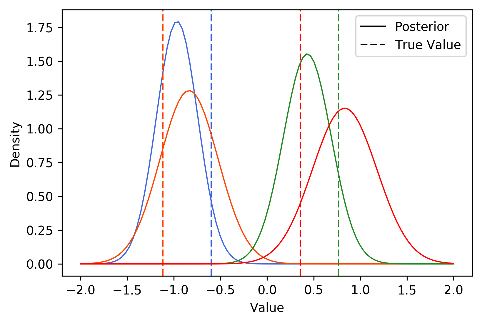
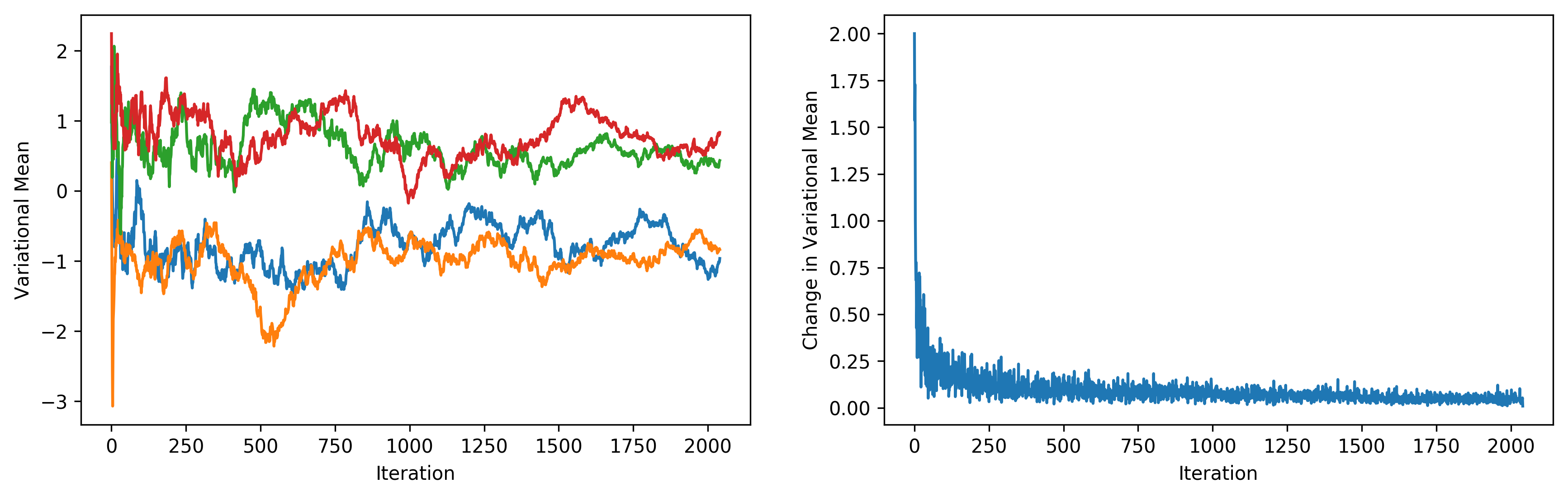
It appears that BBVI does a pretty decent job of picking up the distribution over true values. The following plots depict the value of each variational mean at every iteration (left), along with the change in variational means (right).
Again, I highly recommend checking out the original paper. This Python tutorial by David Duvenaud and Ryan Adams, which uses BBVI to train Bayesian neural networks in only a few lines of Python code, is also a great resource.
All my code is available here.