Lies, Damned Lies, and Causal Inference
Published:
To paraphrase Benjamin Disraeli, statistics makes it easy to lie. In this post, I’ll go over an example from Judea Pearl’s excellent textbook, Causality, that shows how different statistical approaches can lead to different estimates of the causal effect of smoking on lung cancer.
First, the (fictional) data, which is taken from Section 3.3 of Causality. Say we have results from an observational (i.e. non-randomized) study, that aims to assess the affect of smoking on developing lung cancer. For every person, we have a binary variable \(X\) that indicates whether that person is a smoker and a binary outcome variable \(Y\) that indicates whether that person developed lung cancer. Additionally, we have a binary variable \(Z\) that indicates whether each person had a significant amount of tar in their lungs.
The results from the (fictional) study are depicted in the table below:
\begin{array}{c|c|c|c} \text{Smoker } (X) & \text{Tar }(Z) & \text{Group Size (% of population)} & \text{Cancer Prevalence (% of group)} \
\hline 0 & 0 & 47.5\% & 10\%\
0 & 1 & 2.5\% & 5\%\
1 & 0 & 2.5\% & 90\%\
1 & 1 & 47.5\% & 85\%\
\end{array}
At first glance, it seems that smoking is likely to cause cancer. Ignoring \(Z\), both groups of \(X = 1\) have a far larger prevalence of cancer than \(X = 0\). Even considering \(Z\), smokers with tar buildup are more likely to have cancer than nonsmokers with tar buildup, and smokers without tar buildup are still more likely to have cancer than nonsmokers without tar buildup.
Indeed, simple calculations using Bayes’ rule verify \(P(Y = 1 \vert X =0) = .10\) and \(P(Y = 1 \vert X = 1) = .85\), indicating one is much more likely to have lung cancer if that person is also a smoker.
However, this might be misleading. The Bayes’ rule calculation above corresponds to a prediction problem: What’s the probability someone has cancer if she’s a smoker? In real life, we may be more curious about the causal problem: What’s the probability that smoking will cause someone to have cancer? The distinction may seem like a subtle one but it’s important. It may be possible that lung cancer and smoking are correlated due to a common cause, but that lung cancer does not directly (or indirectly) cause smoking. Since we’re concerned with an intervention (i.e. choosing to smoke or not), we would like to estimate the direct cause of this intervention.
This problem came up in a causal inference class I’m taking this semester, and our professor likes to say it’s easy to go down philosophical rabbit holes when defining causality. I’ll leave that to the experts (there are excellent textbooks by Guido Imbens and Don Rubin along with Stephen Morgan and Christopher Winship).
An intuitive approach for me is through the use of causal graphs. I won’t go over all the details, but the main idea is that every node in the graph represents a variable in the causal problem of interest, and the arrows between each node show the causal direction. Nodes can either be observed (shaded) or latent (unshaded).
For example, in the smoking example, we would depict \(X\), \(Y\), and \(Z\) with observed nodes. It’s fair to imagine that the decision to smoke will cause the amount of tar buildup in the lungs, and we can also assume that lung cancer is only caused by tar in the lungs. In this case, we would have an arrow from \(X\) to \(Z\) followed by another arrow from \(Z\) to \(Y\).
This is unrealistic, however, as there are likely unknown, unobserved causes that confound these variables. For example, genetics can influence our decision to smoke, and it can also determine our predisposition to cancer. It wouldn’t be a stretch to assume that tar buildup is determined only by smoking. (These assumptions are definitely simplifying and unrealistic, but that’s besides the point for this example.) Accounting for this confounder illuminates the difficulties posed by the causal approach: people who are genetically inclined to smoke may also be more genetically likely to have cancer, correlating these two variables without a causal relationship.
Denoting genetics as the latent variable \(U\), the causal graph is depicted in subfigure (a) below:
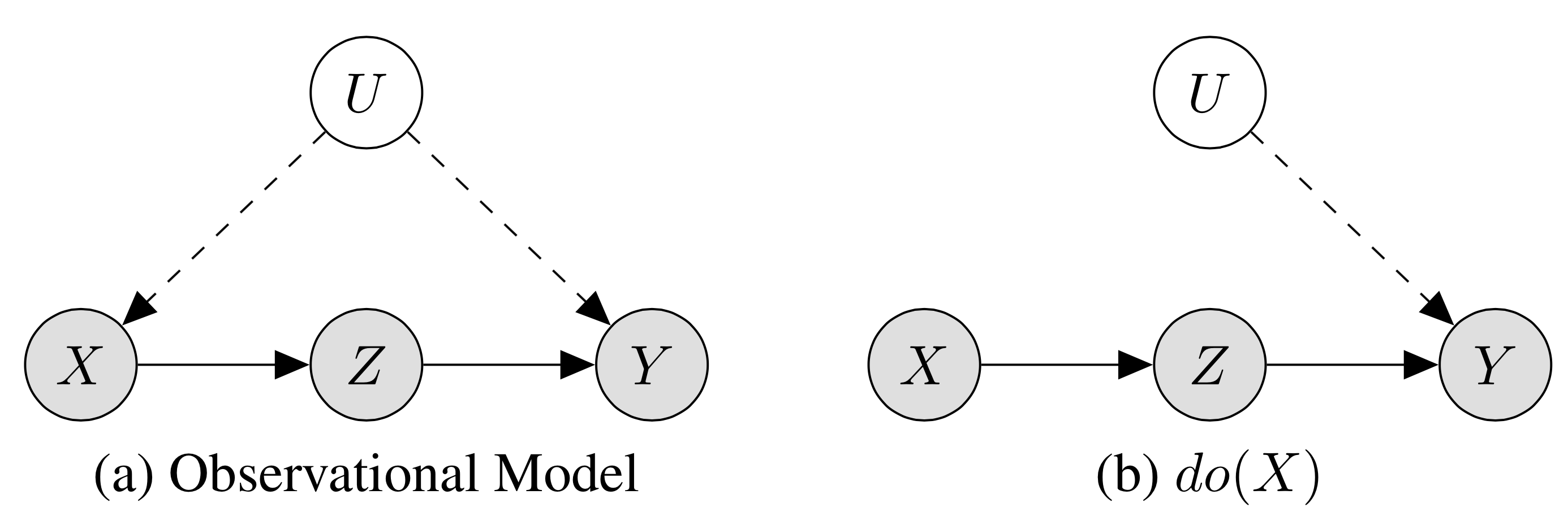
If we’re interested in the causal effect of \(X\) on \(Z\), we are thinking in terms of interventions; that is, \(X\) would no longer depend on \(U\) if someone is forced to smoke or to not smoke. Thus, Pearl introduces the \(do(\cdot)\) operator, which imagines the causal graph under intervention. If \(do(X = 1)\), we force \(X\) to be 1, and imagine that \(X\) is only caused by the “do-er” as opposed to any of its causal predecessors, since we can intervene. Thus, the causal effect of interest becomes \(P(Y = 1 \vert do(X = 1))\) as opposed to \(P(Y = 1 \vert X = 1)\). This scenario is depicted in subfigure (b) above.
Because of the confounding variable \(U\), the numbers at the beginning of this post do not accurately reflect the causal effect. There are several set of criteria for calculating causal effects based off causal graphs, most notably the back-door and front-door criteria. Using the front-door criterion (which I won’t elaborate on here but deserves its own post), we can see that \(Z\) is an intermediate causal effect. That is, \(Z\) only depends on \(X\) through \(X\).
We can then calculate the effect of \(Z\) on \(Y\); however, there exists what’s called a back-door path from \(Z\) to \(Y\) through \(X\). That is, if we just calculate the causal effect of \(Z\) on \(Y\), because of the confounder \(U\), we would include spurious effects that are due to \(X\). Therefore, we must block \(X\) by accounting for it when calculating the causal effect. Chapter 3.3 of Pearl’s textbook goes through these derivations in more depth.
Mathematically, then, we can calculate
\[P(Y = 1 \vert do(X = x)) = \sum_{z=0}^1 P(Z = z \vert X = x) \sum_{x'=0}^{1} P(Y = 1 \vert X = x', Z = z)P(X = x').\]The \(P(Z = z \vert X = x)\) term accounts for the intermediate causal effect of \(X\) on \(Z\). The term in the sum estimates \(P(y = 1 \vert do(Z = z))\) by conditioning on \(X\) to account for the final causal effect of \(Z\) on \(Y\). Using this formula with the same data (re-posted below), we can calculate \(P(Y = 1 \vert do(X = 1)) = 0.45\) and \(P(Y = 1 \vert do(X = 0)) = 0.50\), indicating that smoking would actually decrease the chance of lung cancer.
Intuitively, what’s going on? It appears that smoking increases the amount of tar buildup in the lungs, which is easily verified in the table below, since \(P(Z = 1 \vert X = 1) = 0.95\) and \(P(Z = 1 \vert X = 0) = 0.05\). However, we can see that conditioning on \(X\), tar buildup decreases your likelihood of getting lung cancer. That is, \(P(Y = 1 \vert X = 1, Z = 0) > P(Y = 1 \vert X = 1, Z =1)\) and \(P(Y = 1 \vert X = 0, Z = 0) > P(Y = 1 \vert X = 0, Z = 1).\) Thus, combining these results: smoking causes a larger amount of tar buildup in the lungs, and large tar buildups in the lungs prevent cancer.
\begin{array}{c|c|c|c} \text{Smoker } (X) & \text{Tar }(Z) & \text{Group Size (% of population)} & \text{Cancer Prevalence (% of group)} \
\hline 0 & 0 & 47.5\% & 10\%\
0 & 1 & 2.5\% & 5\%\
1 & 0 & 2.5\% & 90\%\
1 & 1 & 47.5\% & 85\%\
\end{array}
I want to stress this data is fictional, and the arguments are simplistic. One could easily come up with another causal diagram to show that smoking increases the likelihood of cancer. However, I think this example illustrates the importance of being careful when performing causal inference analyses, along with the differences between causal inference and prediction problems.